


Long Term Behavior
In the lectures, we developed a model for the growth of a population based on the assumption that the growth rate over a period is based on the current size of the population.
$$\Delta a_{n+1} = ka_n$$ $$a_{n+1} = (1+k)a_n = ra_n$$ $$a_n = a_0 r^n$$When we're thinking about models like this, it's useful to think about how it behaves in the long term, i.e. for large values of $n$, for different values of its parameters.
$a_0$, the initial population has size is constant and has to be greater than or equal to 1 so it's affect is only going to scale the results. For example, a value of 100 will make the population values change 10 times faster than a value of 10 but it won't change the over all direction or behavior. Since all we're interested in is that behavior, we can chose a reasonable value for $a_0$, say 50, and start analyzing the behavior for different values of $r$ from there.
For each of the following ranges of $r$, pick several values (where appropriate), come up with a numeric solution, graph each one then suggest what the long term behavior is for values in that range.
- $r > 1$

- $r = 1$ or $r = 0$
- $0 < r < 1$
- $r < 0$
The results are summarized below. Click on the box to display the text once you're done with your calculations.
I choose $r=1.5, 3\text{ and } 5$ and got the following results. In the first table, I left out the larger values for $r= 3$ and $r=5$ since those graphs grow so fast it quickly became impossible to see the behavior of the $r=1.5$ scenario. The second graph shows the complete sequences for all three options. This is enough for us to conclude that the population becomes unbounded for values of $r > 1$.


| n \ r | 1.5 | 3 | 5 |
| 0 | 50 | 50 | 50 |
| 1 | 75 | 150 | 250 |
| 2 | 112.5 | 450 | 1250 |
| 3 | 168.75 | 1350 | 6250 |
| 4 | 253.125 | 4050 | 31250 |
| 5 | 379.6875 | 12150 | 156250 |
| 6 | 569.53125 | 36450 | 781250 |
| 7 | 854.296875 | 109350 | 3906250 |
| 8 | 1281.4453125 | 328050 | 19531250 |
When $r=1$, the sequence becomes $a_n=a_0$ for all $n$ and when $r=0$, it becomes $a_n=0$ also for all $n$, i.e. it's constant in both cases.
I choose $r=.75, .5\text{ and } .25$ and got the following results. You can see in all three cases that the population is dropping off to 0 so we've found a circumstance where it will eventually go extinct.
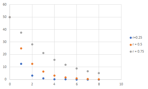
| n \ r | 0.25 | 0.5 | 0.75 |
| 0 | 50.000 | 50.000 | 50.000 |
| 1 | 12.500 | 25.000 | 37.500 |
| 2 | 3.125 | 12.500 | 28.125 |
| 3 | 0.781 | 6.250 | 21.094 |
| 4 | 0.195 | 3.125 | 15.820 |
| 5 | 0.049 | 1.563 | 11.865 |
| 6 | 0.012 | 0.781 | 8.899 |
| 7 | 0.003 | 0.391 | 6.674 |
| 8 | 0.001 | 0.195 | 5.006 |
I choose $r=-1.5, -1\text{ and } -0.5$ and got the following results. I added lines connecting the points to make the behavior clearer. In all three cases, we're seeing the same general behavior that we saw with the corresponding positive $r$ values only oscillating between positive and negative. This is clearly an unrealistic behavior for a physical population so we would normally not allow $r$ values in this range.
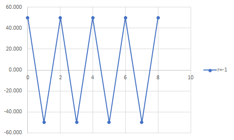
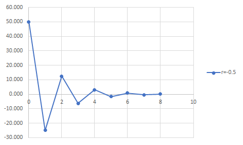
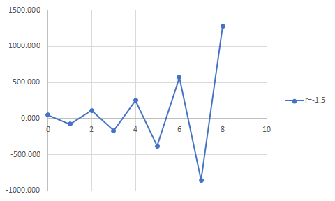
| n \ r | -0.5 | -1.0 | -1.5 |
| 0 | 50.000 | 50.000 | 50.000 |
| 1 | -25.000 | -50.000 | -75.000 |
| 2 | 12.500 | 50.000 | 112.500 |
| 3 | -6.250 | -50.000 | -168.750 |
| 4 | 3.125 | 50.000 | 253.125 |
| 5 | -1.563 | -50.000 | -379.688 |
| 6 | 0.781 | 50.000 | 569.531 |
| 7 | -0.391 | -50.000 | -854.297 |
| 8 | 0.195 | 50.000 | 1281.445 |
